the Creative Commons Attribution 4.0 License.
the Creative Commons Attribution 4.0 License.
 | 04 May 2022
What can we see from the road? Applications of a cumulative viewshed analysis on a US state highway network
In many parts of the world, motorized travel is one of the most common ways that people interact with their regional landscape. This study investigates how travelers' understandings of place might be influenced by what landforms they can see from a vehicle. It uses a cumulative viewshed analysis on the Washington State (United States) highway network to determine which physical landscape features are most frequently visible or obscured from the road. Adapting ideas from Kevin Lynch's The Image of the City, I propose spatial data processing methods to derive landmarks, edges, and districts that could most contribute to the mental maps of travelers and should be prioritized for labeling on print, electronic, and augmented reality maps. Other applications of the cumulative viewshed include deriving scenic byways, siting proposed construction for high or low visibility, and guiding conversations about critical toponymy and perceptions of place.
- Article
(15497 KB) - Full-text XML
-
Supplement
(54 KB) - BibTeX
- EndNote


In many areas of the world, motorized travel on cars, buses, motorcycles, and other vehicles is the primary way that people move between locations in their home regions. Traveling along the highway, they take in a visual panorama that includes landforms moving through the field of view in an ever-changing display (Cron, 1959, p. 88; Lowenthal, 1978). Indeed, this is one aspect of automobile travel that many motorists find enjoyable. “The view from the road can be a dramatic play of space and motion, of light and texture, all on a new scale,” observed Appleyard et al. in 1964 (pp. 3–4). Even for urban commuters who get no thrill from sitting in traffic, motorized travel is still one of the most common ways to see the natural landscape.
Although there are various sensory ways to learn and know a landscape, such as sounds and smells, the motorist is largely sealed off from these, primarily relying on vision. Scenes from the highway influence the ways that motorists perceive space and orient themselves. Traveling through a place can reduce ignorance of that landscape for passengers who are attentive and traveling during daylight (McKenna et al., 2008). No longer terra incognita, the roadside landscape might even take on an outsized role in motorists' understandings of place. People's mental maps tend to exaggerate the size, prominence, and frequency of features that they have seen or interacted with (Gould and White, 1974, p. 33, p. 130).
That being said, mechanized travel allows only a rapid and relatively limited set of views, viewpoints, and angles compared to those that would be available if the observer could simply roam the landscape, a fact sometimes bemoaned by early rail travelers (Schivelbusch, 1986). The appearances of natural features from the roadway are likewise constrained and further affected by environmental factors such as weather and lighting (Unwin, 1975). Even with the possibility of motorized travel, our cognitive maps sometimes remain sketchy and impressionistic. As our mental maps grow through repeated exposure and experiences, so expands our set of behavioral options, sense of security, and feelings of enjoyment and meaning in the landscape (Bell et al., 1978, pp. 267–269; Chang et al., 2019).
For decades, urban planners and landscape architects have sought to understand how pedestrians and motorists interpret and navigate cities from streets and sidewalks. I propose that some of these inquiries can help learn how people perceive the natural landscape of the broader region. The volume The Image of the City of Lynch (1960) posited that our environmental image
is the product both of immediate sensation and of the memory of past experience, and it is used to interpret information and to guide action. The need to recognize and pattern our surroundings is so crucial, and has such long roots in the past, that this image has wide practical and emotional importance to the individual. (Lynch, 1960, p. 4)
A clear mental image of a landscape is thus the starting point for further learning, exploration, and individual growth.
By studying residents' mental maps and navigation habits among three US metropolises, Lynch developed a framework of five elements that contribute to people's image of the city. These are paths, edges, districts, nodes, and landmarks. Paths are channels of movement, such as roads and railways; edges are other linear elements not used as paths, such as shorelines or walls; districts are areal units with a common identifying character, such as neighborhoods; nodes are strategic foci of travel such as stations and junctions; and landmarks are point references not participating in the travel network, such as hilltops or distinctive skyscrapers (Lynch, 1960, pp. 46–48).
The density at which these elements are perceived on the cityscape determines the legibility and imageability of the landscape. For example, participants in Lynch's study had a well-developed image of the city of Boston along the Charles River where edges, paths, and landmarks were abundant and markedly defined; but the details of their understanding declined with distance from the river's edge. Some neighborhoods were even difficult for their own residents to conceptualize due to irregular street matrices and scarcity of landmarks (Lynch, 1960, p. 20).
At the state or provincial scale, features such as roads, ridges, basins, cities, and peaks all find corollaries in Lynch's framework. The degree to which these features actually do fill the roles of paths, edges, districts, nodes, and landmarks is partly based on how visible they are (McKenna et al., 2008). In this context, GIS-based visibility analysis becomes useful for determining which landforms and other natural features might contribute most to the legibility of the landscape.
As computer processing power has improved over the years, some researchers have explored whether Lynch's elements can be derived from spatial databases using algorithms. Computation was viewed as an attractive circumvention of the time and cost associated with finding and interviewing residents about their mental maps. Campagna et al. (2012), for example, experimented with finding prominent paths based on size and topological connectivity of streets, but only after noting that some of Lynch's elements are defined by personal, historical, or cultural meanings that might be harder to calculate.
Other studies introduced visual properties into the computation of Lynchian elements. Dalton and Bafna (2003) used ideas from space syntax research, such as axial lines and isovists (eye-level cross-section polygons of the field of view). The latter were useful for detecting edges, although the authors felt that the “visual elements” of edges and landmarks played only a secondary role of fine-tuning the mental map when compared with the “spatial elements” (nodes, paths, and districts) that the subject could actually traverse. Morello and Ratti (2009) used a digital elevation model (DEM) and employed 3D isovists to calculate Lynchian elements as the subject traveled through urban space. Their work uses cumulative isovists to understand commonly visible surfaces. Filomena et al. (2019) proposed methods for computing all five of Lynch's elements, identifying landmarks by measuring building heights and the longest lines of sight. They also looked at nearby points from historic registries in an attempt to capture some of the socio-cultural meaning associated with the potential landmarks.
Some have questioned how much Lynch's elements are still relevant in the digital era. Park and Evans (2018) note that digital wayfinding tools can elevate alternative routes that might have once been secondary or tertiary in nature (for example, to get around accidents or slowdowns), thereby muddying the clear spatial hierarchy of path structures advocated by Lynch. Hamilton et al. (2014) observe that as algorithms generate maps dynamically, the traveler has less need of a cognitive map or wayfinding skills. Out of Lynch's five elements, this development has the biggest effect on landmarks. Indeed, the definitive landmark in the algorithmic city may actually be the self.
The present article contemplates what Lynch's elements might look like when applied to geomorphological features on a state-level scale and explores ways of identifying possible elements using visibility analysis. Since Lynch's framework was developed in cities, some aspects of it may not translate directly to rural settings; for example, in the countryside, the path network is more limited than in the city. There may only be one reasonable way to get between an origin and destination point. Similarly, nodes as critical junctions between paths may be fewer and farther between. Some elements may not be used directly for route-finding but still contribute to travelers' mental maps and understanding of relative positioning. In the natural landscape setting, the visual elements of edges and landmarks identified by Dalton and Bafna (2003) are useful toward personal orientation and confirming a sense of place. Districts are also possible to derive as polygonal areas that can be seen and comprehended. Thus, the present analysis focuses on identifying landmarks, edges, and districts.
GIS offers numerous approaches for studying the areas that are visible from any particular vantage point. Gridded (raster) data are most common in these analyses, wherein each cell value represents the elevation of the terrain. The software performs geometric calculations on this “digital elevation model” (DEM) to systematically detect whether anything is blocking the view between the observer cell and all possible target cells (Travis et al., 1975; Fisher, 1991). The set of cells visible from the input observer cell is commonly referred to as the viewshed of the input cell. Viewsheds have been deployed in landscape planning (Travis et al., 1975; Fisher, 1996; Sander and Manson, 2007), tourism and recreation studies (Wilson et al., 2008; Jakab and Petluš, 2013), historical analysis (Randle, 2011), and many other fields.
The most accurate method of deriving a viewshed is to calculate the line of sight between the observer cell and all other cells in the study area; however, this approach is time-consuming. Algorithms that make relatively minor sacrifices in accuracy can shorten the processing time considerably by strategically reducing the number of sight lines calculated. Ways of doing this include calculating the lines of sight to the grid edge cells first and using the results to estimate values of inner cells, or working outward from the observer in concentric rings in a way that skips calculations on areas already estimated to be obstructed (Franklin and Ray, 1994; De Floriani and Magillo, 2003; Kaučič and Zalik, 2002; Carver and Washtell, 2012). A different method described by Wang et al. (2000) avoids sightlines and instead uses “reference planes” defined by the heights of the observer cell and two other cells just in front of the target cell. This is the algorithm employed in the free and open-source Geospatial Data Abstraction Library (GDAL) software (Warmerdam, 2008). It was chosen for the present study due to its free and widespread availability, transparent documentation, and reasonable speed.
A viewshed of a single point can be recorded in a Boolean raster format using a value of 1 to denote cells within the viewshed and 0 or “no data” values for all other cells. When viewsheds are calculated from multiple points, the resulting layers can be summed to create a cumulative viewshed wherein the value of any given cell represents the number of observer points that can see that cell. For example, Wheatley (1995) used a cumulative viewshed analysis (CVA) to map how many archeological monuments were visible from any vantage point within an area of interest. The study also examined the cumulative viewshed counts at the monument points themselves to help determine if intervisibility might have been a factor in monument placement.
Determining visibility from polyline features (such as a road network) is carried out in practice by placing points at a fixed interval along the lines and creating a cumulative viewshed from those points. Chamberlain and Meitner (2013) gave an example of this approach to determine scenery visible from a 6 km segment of highway, with the sample points placed about 10 m apart. They described several variations on this technique to account for the speed of the vehicle and the visual magnitude of the feature within the motorist's field of view. Lee and Stucky (1998) used cumulative viewsheds as a cost surface to determine ideal paths for a variety of scenarios such as keeping unsightly features out of view, maximizing scenic vistas, and conducting reconnaissance.
Some probes of novel viewshed methods have been limited by computational capacity, especially when generating many viewsheds over a broad landscape. Most studies involve urban areas or small rural study sites. For example, when calculating visibility from a sample of 220 residential properties within a town, Sander and Manson (2007) mention limited computing time as a barrier to a more comprehensive inquiry. Today's increased computational capacity and data storage capacities can allow for broader CVA studies across states or countries, especially when the viewsheds are generated and summed through automated scripts.
The present study takes advantage of automation to generate and sum many thousands of viewsheds along the highways of Washington State, a study area of approximately 184 000 km2 in the northwestern corner of the contiguous United States. A variation on the analysis weights the viewsheds by traffic counts to get a better understanding of the features visible to the most highway travelers. The results from these cumulative viewsheds are used to construct elements from Lynch's framework, thereby getting a feel for which geographic features might contribute most heavily to motorists' readings of the landscape. I conclude the analysis by discussing different uses of the cumulative viewshed, as well as some of the limitations involved in this approach.
The set of 1 arcsec DEMs covering Washington State was downloaded from the United States Geological Survey (USGS) National Map downloader website (https://apps.nationalmap.gov/downloader/#/, last access: 28 April 2022). The author projected these DEMs into UTM Zone 10 N, mosaicked them, and clipped them to the official state boundary (including water). The cells' spatial resolution of approximately 30 m was fine enough to capture the visibility of major natural features, while being coarse enough to allow for the calculation of thousands of viewshed operations across long distances. For more localized analyses not involving an entire state, a higher-resolution DEM would be preferable.
Highway polylines containing average annual daily traffic (AADT) counts for the year 2019 were obtained from the Washington Geospatial Open Data Portal (https://geo.wa.gov/search, last access: 28 April 2022). This dataset is maintained by the Washington State Department of Transportation and contains all numbered federal and state highways within Washington State, totaling about 11 362 km in length.
The traffic counts were reported as attributes of these polyline segments. Multiple segments made up a single highway, with the counts varying up and down along each route according to how many vehicles per day were estimated to travel the road on average during 2019. More recent counts were not sought, due to the influence of the COVID-19 pandemic on typical traffic patterns.
To prepare for the viewshed generation, the highways were joined by their route numbers, and a set of sample viewpoints was generated at 1 km intervals along each route. Points known to be in tunnels were discarded. The traffic counts from the original highway segments were then spatially joined onto the viewpoints. This created a dataset with 11 225 viewpoints, each containing a traffic count estimate.
3.1 Procedure for generating cumulative viewsheds
Using a Python script (S1) and the open-source GDAL processing library, a viewshed was generated for each viewpoint. During this computation, a 1 m vertical offset was added to each viewpoint elevation to represent the minimum reasonable height of an individual looking out of a vehicle (Smith, 2006, p. 144; Capaldo, 2012). An earth curvature coefficient of 0.85417 was applied as suggested in the GDAL documentation. Visible cells were coded as 1, and other cells were coded as 0.
Additionally, a second version of the viewshed was weighted by the AADT count. In other words, if a viewpoint had an AADT count of 5000 vehicles, all visible cells were coded as 5000, and non-visible cells were coded as 0. Both the weighted and unweighted viewsheds were saved as compressed TIFs.
The entire process of creating the viewshed, making a weighted copy, and compressing the results took an average of 38 s per viewpoint using an Intel i7-6700 CPU running at 3.40 GHz with 64 GB of RAM. Distribution of the task across multiple machines could reduce the processing time if needed. The unweighted Boolean viewsheds were summed one by one using the GDAL Calc operation in order to obtain the cumulative viewshed in Fig. 1. In this map layer, the value of each cell represents the number of viewpoints that can see that cell.

Figure 1Cumulative viewshed showing the number of sample viewpoints that can see each cell. The highway network used for analysis is included, along with some other geographic features for context.

Figure 2Cumulative viewshed weighted by average annual daily traffic count. The cell value represents the total traffic count from all sample viewpoints that can see the cell.
The traffic-weighted viewsheds were also summed to create a cumulative viewshed representing how much traffic at the viewpoints could see each cell during an average day (Fig. 2). Note that these cell values do not directly translate into how many people see the cell each day, as many people's trips may span multiple points and there are often multiple people within a single vehicle; however, they do help indicate which geographic features are visible to the most travelers.
Note that these methods could be used on part of the data in order to answer certain questions. For example, cumulative viewshed methods can show all the land visible from one particular highway. To demonstrate this, Fig. 3 combines all the viewsheds along Interstate 90, the main east–west thoroughfare through the state connecting its two largest cities of Seattle and Spokane. In this map, pixels are simply classified as visible or invisible to give the viewer a quick and easy feel for which features a motorist could see.

Figure 3Area visible from Interstate 90, the main east–west artery through Washington State.
3.2 Procedure for identifying landmarks and edges
The resulting cumulative viewsheds are quite detailed. They can be used “as is” for a city- or county-level analysis, but visualizing patterns at the state level requires some smoothing and generalization. The following procedure was used to isolate the most visible peaks and ranges using spatial data processing algorithms, thereby serving as a guide for digitizing Lynchian landmarks and edges.
-
Each cell in the cumulative viewshed was recoded with the maximum cell value falling within a radius of 1 km. The result of this was then downsampled to a 1 km cell size for faster processing and easier visual interpretation.
-
The top 5 % of pixels with non-zero values (in this case, those visible from 153 or more points) were extracted into a Boolean raster and converted into polygons.
-
A spatial aggregation operation was performed to combine any polygons with less than a 5 km gap between them, while removing any polygons or holes of fewer than 25 km2.
-
(Optional) To further narrow the results, for any polygon not containing a pixel in the top 1 % of non-zero cells, the Step 1 result raster was discarded. (In this case, polygons visible from fewer than 380 viewpoints were removed.)
The resulting polygons represent some of the most widely visible ridges, ranges, and peaks. They can be used as a cartographic aid for digitizing Lynchian edges and landmarks, an approach that is more objective than simply eyeballing the raw results from the cumulative viewshed. Employing the algorithmically derived patterns in tandem with the cartographer's local knowledge, experience, and supplemental map layers results in a more meaningful set of features than could be obtained by the computer or human alone.
3.3 Procedure for identifying districts
A similar procedure was used to derive districts as areas that the user enters “inside of” whose relatively high visibility facilitates the mental construction of a “common, identifying character” (Lynch, 1960, p. 47). Since so many of the highly visible pixels in the cumulative viewshed layer were in rugged and mountainous areas that would be difficult to traverse, the calculation of districts presented here focuses on separating out the flatter areas that are still highly visible.
- 1.
A slope layer of the DEM was smoothed by recoding each cell with the median value within a 1 km radius. The result was resampled to a 1 km cell size for faster processing and easier visual interpretation.
- 2.
The unweighted cumulative viewshed was also smoothed by recoding each cell with the median value within a 1 km radius and rounding it to an integer. The result was resampled to a 1 km cell size for faster processing and easier visual interpretation.
- 3.
Using the raster layer produced in Steps 1 and 2, a new layer was made containing only cells that met both of the following criteria:
-
number of viewpoints visible was in the top quartile of cells (in this case, over 10 viewpoints) and
-
slope was between 0.2 % and 2 % (this captured flatter terrain while eliminating water).
-
- 4.
Qualifying cells were then converted to polygons, and an aggregation operation was applied to generalize the shapes. Any polygons with less than a 5 km gap between them were combined, while polygons or holes of fewer than 25 km2 were removed.
- 5.
Remaining polygons with over 30 km of highway inside were then identified as district candidates, thereby ensuring that these areas were indeed locations of substantial travel. This number of kilometers could be raised or lowered as desired in order to widen or narrow results.
These shapes were used as a guide for human digitizing of the final district polygons in a way that was sensitive to local topographic features. Figure 4 shows how the processing operations described in Sect. 3.2 and 3.3 guided the positioning and orientation of the nodes, landmarks, and edges digitized by the author.
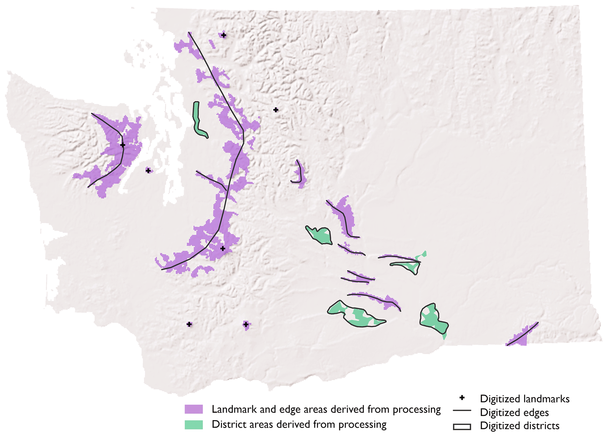
Figure 4Map showing how the landmark, edge, and district candidate areas derived from spatial data processing methods were used as a guide for digitizing the final elements.
The unweighted cumulative viewshed (Fig. 1) shows that the most visible spot of ground from Washington State highways is a location approximately 4298 m high on the northwest flank of Mount Rainier, the highest mountain in Washington State. This pixel is visible from 2104 of the sample points. It might surprise some that the most visible location is not actually the summit of Rainier; however, this is consistent with the Kim et al. (2004) findings that ridges sometimes offer better visibility than peaks.
All sides of Mount Rainier can be seen from state highways. Large sections of the northwest face pointing toward the Seattle area were visible from over 1000 sample points. The only other landforms reaching this threshold were several peaks in the Olympic Mountains, with the most visible being Mount Constance. The high number of viewpoints recorded for these peaks may be due to their visibility from the Seattle and Tacoma metropolitan areas, where there are the most residents and roads. These cities include gentle slopes and expanses of water that afford better views of faraway points.
In the more sparsely populated central part of the state, the Wenatchee Mountains and Rattlesnake Hills are widely seen, as well as long east–west ridges from the Yakima Folds (Kelsey et al., 2017). On the far east side of the state, the Blue Mountains are the most visible. Although the major eastern city of Spokane sits adjacent to several mountain peaks, these are not prominent in the unweighted viewshed, perhaps because of the hilliness of the terrain and edge effects associated with the city being located next to the state boundary.
When the viewsheds are weighted by traffic counts (Fig. 2), the general patterns are similar, although features near metro areas and busy interstate highways are emphasized. These include Mount Spokane, as well as the highlands east of Seattle sometimes locally called the “Issaquah Alps”. In central Washington, the eastern slopes of the Wenatchee Mountains see high values in the weighted cumulative viewshed. These highlands are the first arm of the Cascade Range visible from Interstate 90 as westbound motorists traverse a 110 km straightaway across the Columbia Basin. In fact, these maps show just how much Washingtonians' perceptions of the Cascade Range might be influenced by travel over Snoqualmie Pass on Interstate 90. This is the main artery for personal and commercial vehicle travel between the two sides of the state. The summit sees an average of 34 000 vehicles per day. Figure 3 shows that the viewshed through the pass is generally less than 10 km wide on clear days. On winter days, one is lucky just to see the roadway.
4.1 Map of landscape legibility with Lynch's elements
With the aid of these cumulative viewsheds and the post-processing procedures described above, I have demarcated some of the more “legible” features on the Washington State landscape that could fit into the Lynch (1960) framework discussed earlier. I interpreted paths as the highways and nodes as the major cities along them. Landmarks are highly visible peaks, while edges are highly visible ranges, fronts, and ridges. Districts are area features that the traveler passes through and whose visibility is relatively high from surrounding points, allowing for easy imageability. These include valleys and other bowl-like features such as basins and estuaries.
The result map showing the legibility of Washington from its highways is shown in Fig. 5. Many of the geographic features discussed earlier are prominent landmarks and edges in this map. The eastern front of the Olympic Mountains and the western front of the Cascade Range clearly bound the Seattle metropolitan region. These ranges are not as easily seen from their opposite sides. That being said, central Washington is generally more legible than other parts of the state due to its long folded anticlines, which are even easier to see in the open shrub–steppe environment. Travelers may find it simpler to orient themselves here than in flat regions such as the northern Columbia Basin or areas of rolling topography such as the Willapa Hills and The Palouse.
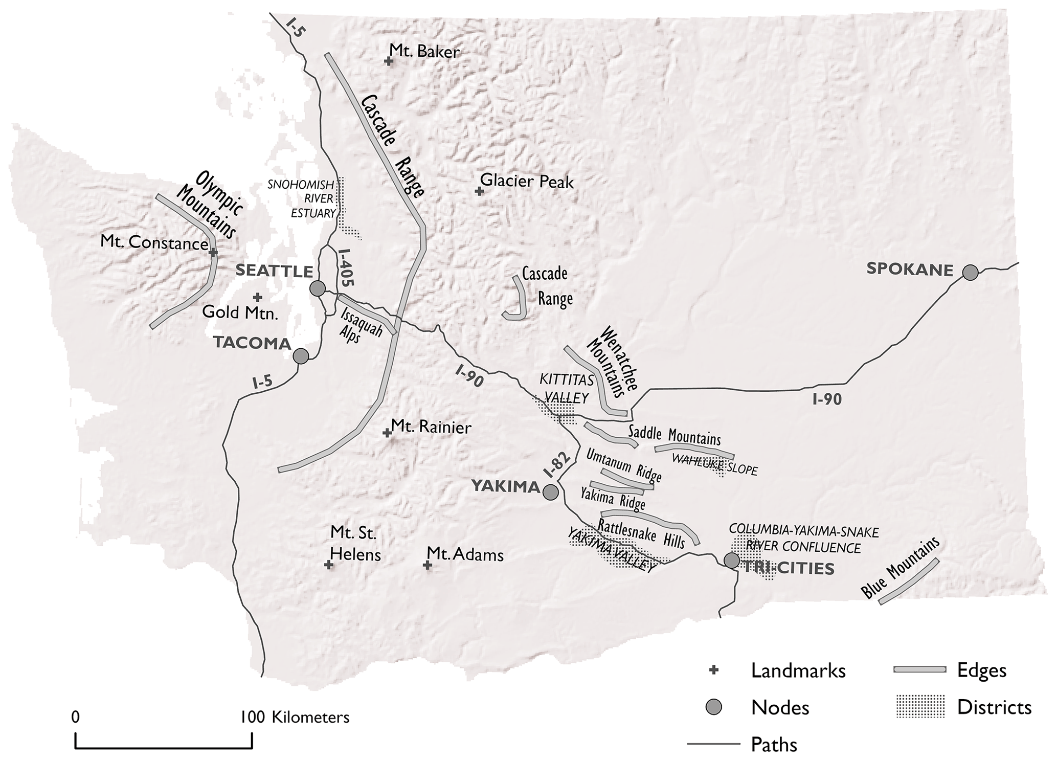
Figure 5Highly visible landmark, edge, and district elements that contribute to landscape legibility, as patterned after Lynch (1960). Nodes and paths are shown as major cities and highways.
What is not easily seen? The interior areas of the Olympic Mountains, including the highest point, Mount Olympus, are not highly visible from the highways. In fact, the cumulative viewsheds show just how much of Washington's mountain ranges motorists cannot see. Residents with good views of the mountains on opposing sides of the Cascade Range (such as in the cities of Seattle or Yakima) may underestimate the breadth of the mountains, as it is sometimes easy to believe that these places lie just “on the other side” of whatever is in the current view. In reality, only a small percentage of the range is visible, with much unseen land lying behind the front.
Areas that are invisible from roads still exist and play important roles in human and environmental systems. Quinn (2020) described some of the activities occurring on “empty spaces” in maps of Washington State, noting that sometimes these were used for NIMBY-type activities that prefer to be kept out of sight and out of mind by urban populations. For example, a person can look at a satellite image all the way back at a 1:7 000 000 scale and still be able to distinguish the Roosevelt Regional Landfill, yet this burial ground for much of the region's trash is not visible from any local road. Much of the commercial forest lands in southwestern Washington that employ clear cuts are both blank on the map and invisible to motorists. Some can be glimpsed from local highways, but the topography blocks the view of much more timberland beyond. The region's economy is highly dependent on these rotational forestry approaches, yet there may be less social license for the clear-cutting practices in landscapes of high visibility.
Observers may also underestimate the scope of agriculture and industry when the majority of the activity falls outside of visible areas. Travelers along eastern Washington's highways are familiar with golden oceans of wheat fields, but there is much more wheat that cannot easily be seen among the famously rolling hills of The Palouse where motorists are generally winding through gullies.
Beyond understanding mental maps, the highway network CVA could be applied in many fields including print and digital cartography, augmented reality development, tourism planning, and toponymic studies.
5.1 Cartography
As people view landforms during their travels, they may ask “What is that?”, perhaps accompanied by the question “Where am I in relation to that?” A glance at popular reference maps shows that some of the most visible landmarks, edges, and districts identified for Washington in Fig. 5 are more commonly labeled than others. At the time of this writing, Google Maps starts showing a few major peaks at zoom level 9. Water bodies such as the Salish Sea also begin to be labeled at this level. As the users zoom in, features and labels go in and out of the view. At zoom level 11, more peaks appear.
In contrast, on OpenStreetMap.org mountains do not appear until level 11, and only then as symbols. Labels for mountains and water features in OpenStreetMap do not appear until level 13. Ranges and ridges are not labeled in OpenStreetMap or Google Maps at any level. One prominent digital map that does show these types of features is Esri's “Topographic” layer, currently the default base map in ArcGIS products.
Print maps are generally better than digital maps at cramming in many labels, including for linear features. When there is only one scale to work with and the label placement is done manually rather than through automated means, cartographers can make rotations, abbreviations, and size adjustments to the text that would be more difficult to achieve through algorithmically generated cartography. This includes curving and stretching a label along the length of a range or ridge. The Rand McNally 2019 Road Atlas page for Washington labels six of the seven landmarks and four of the nine edges (excluding repeats) identified in Fig. 5 (Rand McNally, 2018). The state highway map published by the Washington State Department of Transportation labels six of the seven landmarks and eight of the nine edges (https://wsdot.wa.gov/travel/printable-maps, last access: 28 April 2022). Both maps do not show Gold Mountain, which lies near a visually busy urban area. The state map labels more edges because it includes minor ridges in the central part of the state.
Both print and digital maps fail to label many area features. The Esri Topographic base map is the only one that includes any valleys. From the districts identified in Sect. 3.3, it includes Kittitas Valley and Yakima Valley, as well as Wahluke Slope. None of the maps label estuaries.
5.2 Landscape planning
Highway-based CVA methods can help with decision-making about where to build certain features or use the land in particular ways. Some types of structures might benefit from high visibility, such as retail establishments hoping to attract passing motorists, patriotic or religious symbols (such as flags and places of worship) that wish to catch people's attention, or communication towers that require a clear line of sight for transmitting signals. When performing a CVA for the siting of these facilities, an offset representing the height of the structure could be added to each terrain cell.
Other types of construction or activities might find it desirable to seek a low-visibility place. Activities that are considered unsightly or politically unpopular, such as resource extraction or the burning of fossil fuels might choose to stay out of view of the highway using methods like the ones proposed by Lee and Stucky (1998), although most motorists are burning these fuels themselves. The same goes for military activities such as certain types of combat training or weapons testing. Finally, some developers of recreational or residential facilities may want to build in places that seem distanced from the busy life of the highway, where their clients do not have to see the motorists.
5.3 Tourism promotion and management
The methods described in this paper can also be used to identify potentially scenic byways for further investigation. Knowing these locations could be useful for tourists, photographers, artists, and officials who want to welcome visitors while protecting the surrounding environment.
Recall that each viewpoint originally resulted in a viewshed raster coded with 1 in visible areas and 0 in non-visible areas. To find scenic places, the total number of visible pixels in each raster was calculated and sorted, thereby revealing the viewpoints from which the most geographic area is visible. Figure 6 shows viewpoints whose viewsheds ranked in the top 1 % of visible land area. Several strings of adjacent points indicate good potential byways near the Salish Sea, Mount Rainier, and several basins and valleys in central Washington. A check of Google Street View for the top points confirmed that many offer scenic vistas, although some views are blocked by built structures, vegetation, and features of highway engineering as discussed in Sect. 6 of this study.
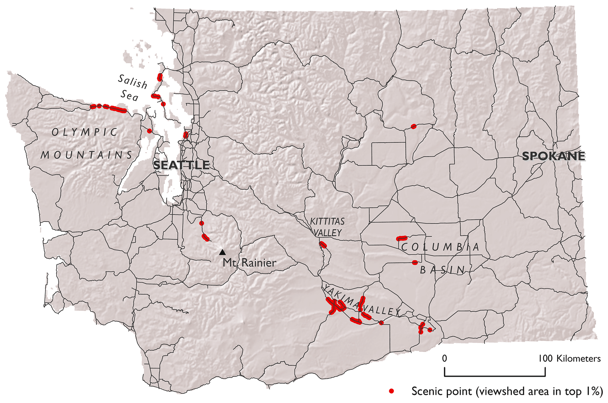
Figure 6Scenic viewpoints identified by taking the top 1 % of sample points in terms of viewshed area.
Points with expansive viewsheds often occur where highways cross or overlook the edges and districts identified in Fig. 5. There are also some highland areas near coasts that offer broad water views. To identify highways that could see the most mountain peaks or other types of features, a CVA could be made based on viewsheds generated at the summits of those landmarks. The values of the cumulative viewshed raster pixels could then be evaluated along the highway sample points (using tools such as Extract Values to Points in ArcGIS or Add Raster Values to Points in SAGA/QGIS) to see which stretches of road had the highest values.
A next step toward confirming the value of these potentially scenic routes would be to consider the types of land use and land cover visible from those locations and how they are perceived and preferred by observers. Strong feelings of meaning, connection, and aesthetic preference could elevate the status of a landmark or other element. Even rural landscapes are laden with symbolic meaning visible in patterns of human appropriation (Cosgrove, 1989), such as agriculture, hydropower, and commercial forestry. Geographers such as Tuan (1990) and Lowenthal (1978) have ruminated extensively on the types of landscape aesthetics preferred by humans. The latter notes that a person's reaction to a landscape may depend on mood, time of day, weather, and modality of travel. Kent (1993) studied reactions to highway scenes and found that patterns of vegetation that allowed some degree of visual penetration facilitated an appealing sense of mystery for travelers. Motorists also positively responded to features that they perceived contributed to the natural or cultural quality of the area, such as unique building architecture.
More recent work has considered aesthetically valued landscapes as “cultural ecosystem services”, attempting to map and understand the non-material benefits that humans derive from landscapes (Plieninger et al., 2013; Bachi et al., 2020). Analysts can use viewshed operations to maximize traveler enjoyment of these landscapes. For example, da Silva et al. (2020) suggested locations for observation towers along a nature trail with the goals of minimizing visual overlap and exposing the hiker to a diverse set of ecosystems. Highway locations with expansive viewsheds could likewise be evaluated for the types of cultural ecosystem services and the variety of landscapes visible to the traveler.
5.4 Augmented reality
The potential for visibility analysis to inform augmented reality applications is vast and still largely untapped. Smartphone apps such as PeakFinder and PeakVisor are popular ways for recreationists to identify what mountain they are seeing just by aiming the phone in the direction of the peak and looking at the display; still, there is an emphasis on point features, with many ridges, ranges, valleys, and basins going unlabeled.
It is easy to imagine asking an onboard navigation system, “What mountain range am I seeing to the right?” and getting an educated guess based on the vehicle's current location and a database of prominent feature names derived from a highway cumulative viewshed. The use of buffers, geo-fences, and individual viewsheds might allow such notices to be actively spoken through the car's speaker system if desired (“now entering the Yakima Valley” or “look to the left and you will see Puget Sound”). One even wonders if an augmented reality windshield display could unobtrusively place labels on ridges, valleys, or water bodies as requested by the driver, thus giving the impression of traveling through the map. The circumstances under which this would be useful, and whether it could be carried out safely, might be a fruitful area for further research.
5.5 Critical toponymy
The landmarks identified in Fig. 5 are visible from vast and diverse areas of the state. Many of these are either stratovolcanos that rise above surrounding mountains or prominent hills seen from across the water. Although they contribute to the everyday landscapes seen by motorists, the origins of the current names of these features do not seem to be widely known by locals. In the northwestern US, it can be easy to forget the relatively recent, and sometimes contested, application of toponyms, or place names. Rose-Redwood et al. (2010) suggest that a critical analysis of the place names we encounter should go beyond individual origin stories and focus on the cultural politics of naming. The most visible features on a landscape seem a suitable place to begin that inquiry.
The observation of Berg (2011) that toponyms are often involved with “settler stories” is largely true for some of the most visible landforms in Washington State, although a more precise name might be “settler government surveyor stories”. The names of Mount Baker and many inland water features in the Salish Sea, such as Puget Sound, come from crew members on the ship of George Vancouver, the first known European to map out the area (Morgan, 1979). Vancouver named Mount Rainier and Mount St. Helens after powerful military and political colleagues back in Britain. Coastal surveyor George Davidson named Mount Constance and nearby peaks “The Brothers” after members of his family (Meany, 1913). In an arm of the Cascade Range highly visible from the east side of the state, George B. McClellan of the U.S. Army gave Mount Stuart the name of a deceased war buddy while making a survey of mountain passes (Meany, 1923, p. 79). The settlers followed these surveyors and inscribed their stories in more place names. They include interest in natural features (Gold Mountain, Glacier Peak), interactions with animals (Rattlesnake Hills), and homage to national heroes (Mount Adams).
On maps (and later in geographic databases), these explorer and settler names replaced ones used by the region's indigenous peoples through centuries past. Although indigenous toponyms generally persist in Washington State to a more prominent degree than in many parts of the country, none of the landmark names in Fig. 5 come from an indigenous language. Failed efforts to rename Mount Rainier with some variation of the indigenous word “Tacoma” played a role in the battle for economic and cultural dominance between the cities of Seattle and Tacoma during the late 1800s and early 1900s (Morgan, 1979, pp. 293–296, 327–328). The effort has been revived by the Puyallup tribe in the wake of the successful decolonial renaming of Denali (formerly Mount McKinley) in Alaska (Sun, 2021). Regardless of the eventual outcome, this attempt will likely provoke more public thought and awareness about the history and meanings of the most visible landform in the state, as well as the ways that place names are applied and contested.
Although this analysis identified some landforms that may be likely to occupy a place in the mental maps of Washington's residents, it did not verify whether the computationally identified landmarks, edges, and districts do indeed play a significant role in people's mental maps. The statewide sampling and outreach that such a verification would entail were deemed to be out of scope of this paper; however, validating computationally derived Lynchian elements with qualitative surveys or other methods such as text mining from books, articles, or conversations would be an informative exercise in future studies.
In order to scale across a broad area with many thousands of viewsheds, this study built upon Boolean visible and invisible calculations carried out on a uniform DEM. The analysis reveals which features should be visible under ideal conditions, but could yield more nuanced results with additional kinds of methods and ground truthing. Features in both the built and natural environments, such as buildings and trees, can obstruct lines of sight and affect the viewshed shapes and areas. This effect can be substantial in heavily wooded areas such as those in western Washington that inspired the nickname “The Evergreen State”. Models that incorporate the heights of built features and forested areas of land cover would give more accurate results, although without enormous amounts of data, they would also be subject to estimation and imprecision.
A viewshed operation is only as accurate as the DEM it is conducted on. Fisher (1991) lists numerous reasons that the actual elevation of a point may differ from its DEM cell value, including problems with the original survey by field workers or photogrammetrists, mistakes by people digitizing these surveys, and poor interpolation. Limitations with the precision of the data format can also hinder accuracy. For example, elements of highway engineering such as cuts through a hillside might obstruct the motorist's view but are sometimes too small to show up in the DEMs used in this study. Higher-resolution DEMs such as those produced with lidar might yield more accurate viewsheds but could increase calculation time to impractical levels. Approaches that use high-resolution data near the highways and a coarser DEM for everything else could also improve accuracy in future experiments (De Floriani and Magillo, 2003). The downside is that these multi-resolution approaches require more data preparation on the front end.
The cloudy and foggy weather associated with the temperate oceanic climate in western Washington often reduces visibility. Parts of the state on the east side of the Cascade Range are generally much sunnier, with clear visibility most of the year. Future studies could factor in weather and climate when determining the most visible features.
Areas shown as invisible in the CVA should be interpreted with caution, since the analysis is based only on viewsheds taken from sample points spaced by 1 km. Stretches of roadway between the sample points might be able to see areas designated as invisible in this CVA. A denser or different set of sample points would yield a different CVA, although not likely different enough to affect the results at a statewide level.
Only areas within the Washington State boundary were considered in this study. Some viewpoints in Washington can see into other states (and Canada), and some viewpoints from those locations are able to see into Washington. Consequently, the values in the cumulative viewsheds and the calculation of the top 1 % of scenic points are subject to edge effects.
Finally, applying strategic weights or functions to the viewsheds might give a better picture of which landforms people see and think about the most often. For example, Mount Rainier takes up much more of the field of view in the city of Tacoma than it does in Yakima. This is because Tacoma is closer to the mountain, sits at a lower elevation, and has fewer other mountains and ridges to obstruct the vista. Approaches that calculate a “visual magnitude” for each cell based on the viewing angle and distance to the target, such as those described by Chamberlain and Meitner (2013), would help with understanding which features take up the most space in observers' fields of view. Carver et al. (2012) attempt to determine visual impact by using an inverse square distance function and the height of the object. Such approaches are more computationally intensive and more complex to interpret than the one described in this paper; however, they may be useful toward better understanding which visible features have the most influence on a traveler's mental map.
Using automated methods, free and open-source software, and fairly ordinary computing power, this study has demonstrated how a cumulative viewshed can be created from a regional highway network traversing well over 100 000 km2. The resulting layer reveals the landforms most widely visible (and invisible) to motorists along the network. Weighting the contributing viewsheds by traffic counts can give a better feel for which areas are visible to the most people. Further spatial data processing on the cumulative viewshed can assist with deriving landmark, edge, and district elements that contribute to people's mental maps as proposed by Lynch (1960).
Cumulative viewsheds derived from highways can help cartographers prioritize features for labeling, especially areal features such as valleys, basins, and estuaries that are often missed. This applies to both print and electronic maps, as well as augmented reality applications that point out geographic features. Other applications of cumulative viewsheds include siting features for high or low visibility, identifying potential scenic byways, and guiding discussions about place names and perceptions.
The Supplement link associated with this paper contains the Python script used to automate the creation of the viewsheds.
The source datasets for this project were downloaded from the US Geological Survey and the state of Washington as described in the methods section (Sect. 3) of this article. The cumulative viewsheds shown in the maps were derived using the code in the Supplement.
The supplement related to this article is available online at: https://doi.org/10.5194/gh-77-165-2022-supplement.
The author has declared that there are no competing interests.
Publisher’s note: Copernicus Publications remains neutral with regard to jurisdictional claims in published maps and institutional affiliations.
The author would like to thank Amanda Moody for her assistance with finding and gathering data for this project and Robert Hickey for providing feedback on the GIS analysis methods.
This paper was edited by Hanna Hilbrandt and reviewed by two anonymous referees.
Appleyard, D., Lynch, K., and Myer, J. R.: The View from the Road, MIT Press, Cambridge, Massachusetts, United States, ISBN 9780262010153, 1964.
Bachi, L., Ribeiro, S. C., Hermes, J., and Saadi, A.: Cultural Ecosystem Services (CES) in landscapes with a tourist vocation: Mapping and modeling the physical landscape components that bring benefits to people in a mountain tourist destination in southeastern Brazil, Tourism Manage., 77, 104017, https://doi.org/10.1016/j.tourman.2019.104017, 2020.
Bell, P. A., Fisher, J. D., and Loomis, R. J.: Environmental Psychology, W.B. Saunders Company, Philadelphia, Pennsylvania, United States, ISBN 9780721617060, 1978.
Berg, L. D.: Banal Naming, Neoliberalism, and Landscapes of Dispossession, ACME: An International Journal for Critical Geographies, 10, 13–22, 2011.
Campagna, M., De Montis, A., Isola, F., Lai, S., Pira, C., and Zoppi, C. (Eds.): Planning Support Tools: Policy analysis, implementation and evaluation, in: Proceedings of the 7th Int. conf. on Informatics and Urban and Regional Planning INPUT 2012, 111–121, https://doi.org/10.48550/arXiv.1212.0940, 2012.
Capaldo, F. S.: Road Sight Design and Driver Eye Height: Experimental Measures, Proc. Soc. Behav., 53, 731–740, https://doi.org/10.1016/j.sbspro.2012.09.923, 2012.
Carver, S. and Washtell, J.: Real-time visibility analysis and rapid viewshed calculation using a voxel- based modelling approach, in: GISRUK 2012 Conference, GISRUK 2012 Conference, 13 April 2012, Lancaster, UK, https://www.geos.ed.ac.uk/~gisteac/proceedingsonline/GISRUK2012/Papers/presentation-48.pdf (last access: 29 April 2022), 2012.
Carver, S., Comber, A., McMorran, R., and Nutter, S.: A GIS model for mapping spatial patterns and distribution of wild land in Scotland, Landscape Urban Plan., 104, 395–409, https://doi.org/10.1016/j.landurbplan.2011.11.016, 2012.
Chamberlain, B. C. and Meitner, M. J.: A route-based visibility analysis for landscape management, Landscape Urban Plan., 111, 13–24, https://doi.org/10.1016/j.landurbplan.2012.12.004, 2013.
Chang, K.-T., Huang, C.-C., and Tsaur, S.-H.: Tourist geographic literacy and its consequences, Tourism Management Perspectives, 29, 131–140, https://doi.org/10.1016/j.tmp.2018.11.005, 2019.
Cosgrove, D.: Geography is Everywhere: Culture and Symbolism in Human Landscapes, in: Horizons in Human Geography, edited by: Gregory, D. and Walford, R., Macmillan Education UK, London, 118–135, https://doi.org/10.1007/978-1-349-19839-9_7, 1989.
Cron, F. W.: The Art of Fitting the Highway to the Landscape, in: The Highway and the Landscape, edited by: Snow, W. B., Rutgers University, New Brunswick, New Jersey, USA, 78–109, 1959.
Dalton, R. C. and Bafna, S.: The syntactical image of the city: A reciprocal definition of spatial elements and spatial systems, in: Proceedings – 4th International Space Syntax Symposium, 17–19 June 2003, London, UK, https://discovery.ucl.ac.uk/id/eprint/1104/1/SIC.pdf.pdf (last access: 29 April 2022), 2003.
da Silva, R. G. P., Henke-Oliveira, C., Ferreira, E. S., Fetter, R., Barbosa, R. G., and Saito, C. H.: Systematic Conservation Planning approach based on viewshed analysis for the definition of strategic points on a visitor trail, International Journal of Geoheritage and Parks, 8, 153–165, https://doi.org/10.1016/j.ijgeop.2020.07.001, 2020.
De Floriani, L. and Magillo, P.: Algorithms for Visibility Computation on Terrains: A Survey, Environ. Plann. B, 30, 709–728, https://doi.org/10.1068/b12979, 2003.
Filomena, G., Verstegen, J. A., and Manley, E.: A computational approach to “The Image of the City”, Cities, 89, 14–25, https://doi.org/10.1016/j.cities.2019.01.006, 2019.
Fisher, P. F.: First Experiments in Viewshed Uncertainty: The Accuracy of the Viewshed Area, Photogramm. Eng. Rem. S., 57, 1321–1327, 1991.
Fisher, P. F.: Extending the Applicability of Viewsheds in Landscape Planning, Photogramm. Eng. Rem. S., 62, 1297–1302, 1996.
Franklin, W. R. and Ray, C.: Higher isn't necessarily better: Visibility algorithms and experiments, in: Vol. 2, Advances in GIS research: sixth international symposium on spatial data handling, Taylor & Francis, Edinburgh, 751–770, 1994.
Gould, P. and White, R.: Mental Maps, Pelican Books, Harmandsworth, Middlesex, England, ISBN 9780140216882, 1974.
Hamilton, K., Karahalios, K., Sandvig, C., and Langbort, C.: The image of the algorithmic city: a research approach, Interact. Design Archit., 20, 61–71, 2014.
Jakab, I. and Petluš, P.: The use of viewshed analysis in creation of maps of potential visual exposure, GIS Ostrava 2013 – Geoinformatics for City Transformation, 21–23 January 2003, Ostrava, Czech Republic, 119–130, http://gisak.vsb.cz/GIS_Ostrava/GIS_Ova_2013/proceedings/print_with_cover.pdf (last access: 29 April 2022), 2013.
Kaučič, B. and Zalik, B.: Comparison of viewshed algorithms on regular spaced points, in: Proceedings of the 18th spring conference on Computer graphics – SCCG '02, the 18th spring conference, 24–27 April 2002, Budmerice, Slovakia, 177–183, https://doi.org/10.1145/584458.584487, 2002.
Kelsey, H. M., Ladinsky, T. C., Staisch, L., Sherrod, B. L., Blakely, R. J., Pratt, T. L., Stephenson, W. J., Odum, J. K., and Wan, E.: The Story of a Yakima Fold and How It Informs Late Neogene and Quaternary Backarc Deformation in the Cascadia Subduction Zone, Manastash Anticline, Washington, USA, Tectonics, 36, 2085–2107, https://doi.org/10.1002/2017TC004558, 2017.
Kent, R. L.: Determining scenic quality along highways: a cognitive approach, Landscape Urban Plan., 27, 29–45, https://doi.org/10.1016/0169-2046(93)90026-A, 1993.
Kim, Y.-H., Rana, S., and Wise, S.: Exploring multiple viewshed analysis using terrain features and optimisation techniques, Comput. Geosci., 30, 1019–1032, https://doi.org/10.1016/j.cageo.2004.07.008, 2004.
Lee, J. and Stucky, D.: On applying viewshed analysis for determining least-cost paths on Digital Elevation Models, Int. J. Geogr. Inform. Sci., 12, 891–905, https://doi.org/10.1080/136588198241554, 1998.
Lowenthal, D.: Finding valued landscapes, Prog. Hum. Geogr., 2, 373–418, https://doi.org/10.1177/030913257800200301, 1978.
Lynch, K.: The Image of the City, MIT Press, Cambridge, Massachusetts, United States, ISBN 9780262120043, 1960.
McKenna, J., Quinn, R., Donnelly, D., and Cooper, J.: Accurate Mental Maps as an Aspect of Local Ecological Knowledge (LEK): A Case Study from Lough Neagh, Northern Ireland, Ecol. Soc., 13, 13, https://doi.org/10.5751/ES-02393-130113, 2008.
Meany, E. S.: The Story of Three Olympic Peaks, The Washington Historical Quarterly, 4, 182–186, 1913.
Meany, E. S.: Origin of Washington Geographic Names, University of Washington Press, Seattle, Washington, United States, https://ir.library.oregonstate.edu/downloads/p5547w38m (last access: 29 April 2022), 1923.
Morello, E. and Ratti, C.: A Digital Image of the City: 3D Isovists in Lynch's Urban Analysis, Environ. Plann. B, 36, 837–853, https://doi.org/10.1068/b34144t, 2009.
Morgan, M.: Puget's Sound: A Narrative of Early Tacoma and the Southern Sound, University of Washington Press, Seattle, Washington, United States, ISBN 9780295956800, 1979.
Park, G. and Evans, G. W.: Lynch's Elements of the City in the Digital Era, J. Am. Plan. Assoc., 84, 276–278, https://doi.org/10.1080/01944363.2018.1524308, 2018.
Plieninger, T., Dijks, S., Oteros-Rozas, E., and Bieling, C.: Assessing, mapping, and quantifying cultural ecosystem services at community level, Land Use Policy, 33, 118–129, https://doi.org/10.1016/j.landusepol.2012.12.013, 2013.
Quinn, S.: Geographies of Empty Spaces on Print and Digital Reference Maps: A Study of Washington State, Cartographic Perspectives, 95, 24–41, https://doi.org/10.14714/CP95.1591, 2020.
Rand McNally: 2019 Road Atlas, Rand McNally, Skokie, Illinois, United States, ISBN 9780528019593, 2018.
Randle, L. B.: Applying the Panopticon Model to Historic Plantation Landscapes through Viewshed Analysis, Historical Geography, 39, 105–127, 2011.
Rose-Redwood, R., Alderman, D., and Azaryahu, M.: Geographies of toponymic inscription: new directions in critical place-name studies, Prog. Hum. Geog., 34, 453–470, https://doi.org/10.1177/0309132509351042, 2010.
Sander, H. A. and Manson, S. M.: Heights and locations of artificial structures in viewshed calculation: How close is close enough?, Landscape Urban Plan., 82, 257–270, https://doi.org/10.1016/j.landurbplan.2007.03.002, 2007.
Schivelbusch, W.: Panoramic Travel, in: The Railway Journey: The Industrialization of Time and Space, University of California Press, Berkeley, California, United States, ISBN 9780520058125, 1986.
Smith, R. F.: State of the Practice and Recommendations on Traffic Control Strategies at Toll Plazas, Prepared by Wilbur Smith Associates for U.S. Department of Transportation Federal Highway Administration, Columbia, South Carolina, United States, https://mutcd.fhwa.dot.gov/rpt/tcstoll/pdf/best_practices.pdf (last access: 29 April 2022), 2006.
Sun, D.: Changing the name of Mount Rainier? The new effort from Washington tribes, KIRO 7 News, https://www.kiro7.com/news/local/changing-name-mount-rainier-new-effort-washington-tribes/RZ7STJVYDNFMLGPNCHZY62CRWI/ (last access: 29 April 2022), 23 April 2021.
Travis, M. R., Elsner, G. H., Iverson, W. D., and Johnson, C. G.: VIEWIT: computation of seen areas, slope, and aspect for land-use planning, US Forest Service Pacific Southwest Forest and Range Experiment Station, Berkeley, California, United States, https://www.fs.fed.us/psw/publications/documents/psw_gtr011/gtr-011part1.pdf (last access: 29 April 2022), 1975.
Tuan, Y.-F.: Topophilia: A Study of Environmental Perceptions, Attitudes, and Values Columbia University Press, New York, New York, United States, ISBN 9780231073950, 1990.
Unwin, K. I.: The Relationship of Observer and Landscape in Landscape Evaluation, T. I. Brit. Geogr., 66, 130–134, https://doi.org/10.2307/621627, 1975.
Wang, J., Robinson, G., and White, K.: Generating Viewsheds without Using Sightlines, Photogram. Eng. Remote Sens., 66, 87–90, 2000.
Warmerdam, F.: The Geospatial Data Abstraction Library, in: Open Source Approaches in Spatial Data Handling, edited by: Hall, G. B. and Leahy, M. G., Springer, Berlin, Heidelberg, 87–104, https://doi.org/10.1007/978-3-540-74831-1_5, 2008.
Wheatley, D.: Cumulative viewshed analysis: a GIS-based method for investigating intervisibility, and its archaeological application, in: Archaeology and Geographic Information Systems: A European Perspective, edited by: Lock, G. R. and Stančič, Z., Taylor & Francis, London, England, 171–186, ISBN 9780748402083, 1995.
Wilson, J., Lindsey, G., and Liu, G.: Viewshed characteristics of urban pedestrian trails, Indianapolis, Indiana, USA, J. Maps, 4, 108–118, https://doi.org/10.4113/jom.2008.1014, 2008.
- Abstract
- Introduction: highway travel and the visible landscape
- Calculating the visible landscape
- Methods
- Results
- Applications
- Limitations and opportunities for further study
- Conclusions
- Code availability
- Data availability
- Competing interests
- Disclaimer
- Acknowledgements
- Review statement
- References
- Supplement